A tensor formalism for computer science
Vespa.ai

WHITEPAPER


A tensor formalism for computer science

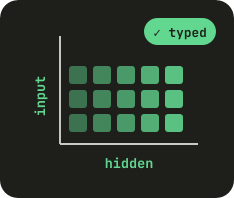
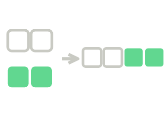
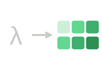
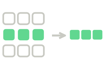
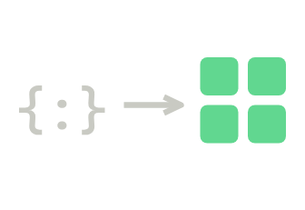
  • Named dimensions
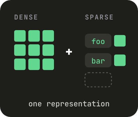
  • Dense + sparse
  • A small, closed set of tensor functions

19 minute read

Isometric drawing of green cubes on a dark grid: a solid block of cells with single outlined cells scattered around it, labelled name{}, {name:bar}, {name:foo} and x[2]
  • Jon Bratseth

    Chief Architect

    Trondheim, Norway

  • Håvard Pettersen

    Sr. Principal Software Engineer

    Trondheim, Norway

  • Lester Solbakken

    Principal Software Engineer

    Trondheim, Norway

International Symposium on Electrical, Electronics and Information Engineering

February 2021

ABSTRACT


Over recent years, tensors have emerged as the preferred data structure for model representation and computation in machine learning. However, current tensor models suffer from a lack of a formal basis, where the tensors are treated as arbitrary multidimensional data processed by a large and ever-growing collection of functions added ad hoc. In this way, tensor frameworks degenerate to programming languages with a curiously cumbersome data model. This paper argues that a more formal basis for tensors and their computation brings important benefits. The proposed formalism is based on 1) a strong type system for tensors with named dimensions, 2) a common model of both dense and sparse tensors, and 3) a small, closed set of tensor functions, providing a general mathematical language in which higher level functions can be expressed.

These features work together to provide ease of use resulting from static type verification with meaningful dimension names, improved interoperability resulting from defining a closed set of just six foundational tensor functions, and better support for performance optimizations resulting from having just a small set of core functions needing low-level optimizations, and higher-level operations being able to work on arbitrary chunks of these functions, as well as from better mathematical properties from using named tensor dimensions without inherent order. The proposed model is implemented as the model inference engine in the Vespa big data serving engine, where it runs various models expressed in this language directly, as well as models expressed in TensorFlow or Onnx formats.

Keywords Computer Science, Machine Learning, Inference

THE FORMALISM

  1. 01 Named dimensions a strong type system for tensors
  2. 02 Dense + sparse, one model a common model of both
  3. 03 A small, closed set of functions a general mathematical language

WHAT IT DELIVERS

  • Ease of use static type verification with meaningful dimension names
  • Interoperability a closed set of just six foundational tensor functions
  • Performance optimization few core functions to optimize · no inherent dimension order

IN PRODUCTION · the model inference engine in Vespa — native, TensorFlow and Onnx models

Figure 1. Three design choices work together to deliver three benefits.

1

Introduction


tensor frameworks degenerate to programming languages with a curiously cumbersome data model.

— ABSTRACT

Tensors - as used in computer science - generalizes scalars, vectors, matrixes and higher-order data structures into a single construct, such that they can be modeled and computed over in a unified way. The adoption of tensors in computer science over recent years in tools such as TensorFlow, NumPy and PyTorch follows the rise of connectionist and numerical approaches in machine learning. The promise of tensors - a concept borrowed from mathematics - is that computation will have a formal basis, enabling operability and meta-computation such as optimization by supplying well-defined semantics, and enabling practitioners to work on a abstraction level than processing of numbers. Has the adoption of tensors delivered on this promise? Arguably not. Taking perhaps the most well-known tensor library, TensorFlow as example, it defines thousands of functions on tensors, many taking parameters specifying their exact behavior, which can only be understood by reading their documentation. It has a separate data model (consisting of multiple dense tensors) for sparse tensors, with separate copies of functions working on them. The lack of support for string indexes has led to string tensor values, which defeats some of the purpose of using a common representation as scalar and string processing is incompatible. Providing full interoperability between TensorFlow and other tools is notoriously hard as new functions and parameters keep being added, and the only precise definition of each function is often the source code.

This paper argues that a more formal basis for tensors based on a strong type system, a common model for sparse and dense tensors, and a small, closed set of universal tensor functions can provide improved usability and interoperability, and provide far better support for optimization.

AD HOC TENSOR FRAMEWORKS

Thousands of functions

  • ×Behavior set by parameters that can only be understood by reading the documentation
  • ×A separate data model for sparse tensors, with separate copies of functions
  • ×No string indexes — so string tensor values, incompatible with scalar processing
  • ×Hard to interoperate; the only precise definition is often the source code

A MORE FORMAL BASIS

A small, closed set

  • ✓A strong type system
  • ✓A common model for sparse and dense tensors
  • ✓A small, closed set of universal tensor functions

→ improved usability and interoperability

→ far better support for optimization

Figure 2. The status quo the paper describes, and the formal basis it proposes in its place.

2

Related work


The difficulty in defining complex computations over tensors based on anonymous indexed tensor dimensions has also been noted by others. Tensor Considered Harmful [1] proposes amending tensors with named dimensions and providing alternatives of operations taking names instead of indexes. Similarly, Tsalib [2] provides a library to add named dimension annotations on top of existing unnamed tensors in current tensor frameworks including Numpy, TensorFlow and PyTorch. AxisArray [3] defines a multidimensional array type used named dimensions for tensor computation in the Julia programming language. These proposals share the idea of using named dimensions to make tensor computations easier to understand with this paper, but none take the opportunity arising from this for creating a small set of generic operations and doing away with dimension ordering, nor do they include support for sparse dimensions.

NAMED DIMENSIONSSMALL SET OF GENERIC OPERATIONSNO DIMENSION ORDERINGSPARSE DIMENSIONS
Tensor Considered Harmful [1]✓
Tsalib [2]✓
AxisArray [3]✓
This paper✓✓✓✓
Figure 3. What each approach covers, as characterized in Section 2.

3

Scope of this paper


  • OUT OF SCOPE

    Function definitions — orthogonal to tensors

  • OUT OF SCOPE

    Mutable tensors — handled by an immutable view during a computation

A practically useful language of computation require a notion of function definitions to provide a way to name and refer to parametrized chunks of computation. A discussion of this is orthogonal to tensors, provided that a pure mathematical notion of computation is used, as here. Therefore, it is left out of this paper.

During learning it is typically necessary to make frequent small adjustments to values in tensors. While this is readily expressed as a join between the tensor under training and an adjustment tensor in the language to be presented here, it requires a notion of a mutable tensor to produce reasonable performance when the trained tensor is large. Mutability is a foreign concept to a mathematical formalism, and so not treated further here, other than noting that mathematically sound computation over a mutable tensor is achieved by providing an immutable view during a computation.

4

Desired features of a tensor formalism


We propose the following desired features of a tensor formalism for computer science:

  • A common representation of dense and sparse tensors. Some machine learning methods use dense dimensions while others use sparse dimensions with an open set of potential points, most which are empty. Furthermore, some combine both kind of dimensions in a single tensor. A general tensor framework need to support both kinds of dimensions, allow them to be combined in a single tensor, and allow computation freely across both kinds. Sparse tensors should support string label indexes to allow strings to be used in models.

  • A strong type system using named dimensions and allowing static type inference of all computation. Named dimensions provide formal documentation that can be semantically verified, making tensor based models easier to work with for humans. In addition, named dimensions allow general computation using a smaller set of core functions having superior mathematical properties (see the next section).

  • A small, closed set of foundational mathematical operations over tensors. With named tensors, it is possible to define a small set of tensor functions in terms of which all other computations can be expressed. This enables interoperability as implementing this small set is all that is needed to realize complete support for tensor computation. Furthermore, it it makes optimization work more efficient as low level optimizations are needed only on this set of functions, while higher-level optimizations can work on whichever chunks of these operations are beneficial, independently of any chunking into higher-level functions humans happen to find meaningful.

5

The tensor formalism


In this section we describe the proposed tensor formalism in full detail, starting with tensors and tensor types, and ending with the set of core tensor functions.

5.1

Tensor types


MAPPED
Sparse. String labels; an open set of points.
INDEXED
Dense. Integer labels 0 … length − 1.
BOUND
An indexed dimension with a size.
ORDER
The number of dimensions in a tensor.

A tensor type consists of a set of dimensions and a value type. The value type is one of the standard numerical types: float, double, etc. The default value type is double.

Each dimension has a name, a type which is either mapped or indexed, and if indexed optionally a size, making it a bound indexed dimension. The number of dimensions in a tensor is called its order. Notice that the notion of a “dimensions” here is separate from “dimensions” in a vector space (where it denotes the length of a 1-dimensional tensor).

A point along a dimension is located by a string or non-negative integer label. Indexed dimensions only use integer labels and must supply values for all integers from 0 to 1 less than the length of the dimension.

All values of a tensor must be located in all dimensions of its type. Values at points which are not explicitly present in a tensor have no default value; they do not exist.

5.1

Tensor types


Diagram titled Anatomy of a tensor type. The type tensor<int>(name{},x[2]) is bracketed into four parts. Tensor type, the tensor keyword. Value type, default double. Mapped dimension, string labels, sparse. Indexed dimension, bound size 2, labels 0 to 1, dense. A bracket over both dimensions reads 2 dimensions, order 2. Enlarge
Figure 4. The parts of a tensor type, using the paper’s own example type.
Diagram titled Anatomy of a tensor type. The type tensor<int>(name{},x[2]) is bracketed into four parts. Tensor type, the tensor keyword. Value type, default double. Mapped dimension, string labels, sparse. Indexed dimension, bound size 2, labels 0 to 1, dense. A bracket over both dimensions reads 2 dimensions, order 2.

A tensor type has a string representation defined by the following (in modernized EBNF):

tensor-type = "tensor" ( "<" value-type ">" )?
                       "(" dimensions ")" ;
value-type = "byte" | "short" | "int" | "long" |
             "half" | "float" | "double" ;
dimensions = | dimension , { "," dimension } ;
dimension = dimension-name ( "{}" | "[" size? "]" ) ;
dimension-name = identifier ;
identifier = [a-zA-Z\_][a-z-A-Z0-9]* ;
size = [1-9][0-9]* ;

Examples:

A double:
tensor()
An indexed, bound vector of 3 floats:
tensor<float>(x[3])
An indexed, bound matrix of unbound x size:
tensor(x[],y[3])
A (sparse) map of named integer values:
tensor<int>(name{})
A map of named vectors of floats:
tensor<int>(name{},x[2])

5.2

Tensors


A tensor consists of a tensor type and a set of values conforming to that type. Only tensors of the 0-order type can have zero values. That tensor is identical to the NaN scalar value.

A tensor has a string representation defined by the following (as a continuation of the EBNF above):

tensor = ( tensor-type ":" )?
         "{" cells | dense-short-form "}" ;
cells = | cell , { "," cell } ;
cell = "{" address "}:" scalar ;
address = | element, { "," element } ;
element = dimension-name ":" label ;
label = integer | identifier ;
dense-short-form =  "[" dense-subspace
                     ( "," dense-subspace )* "]" ;
dense-subspace = dense-short-form | scalar ;

Examples:

A double:
tensor():3.0
An indexed bound vector of 3 floats (dense form):
tensor<float>(x[3]):[0.5, 1, 1.5]
An indexed bound matrix of doubles (dense form):
tensor(x[2],y[3]):[[1.0, 2.0, 3.0], [4.0, 5.0, 6.0]]
A (sparse) map of named integer values:
tensor<int>(name{}):
  { {name:foo}:2, {name:bar}:5 }
A map of named vectors of floats:
tensor<int>(name{},x[2]):
  { {name:foo,x:0}:1,
    {name:foo,x:1}:2,
    {name:bar,x:0}:3,
    {name:bar,x:1}:4 }
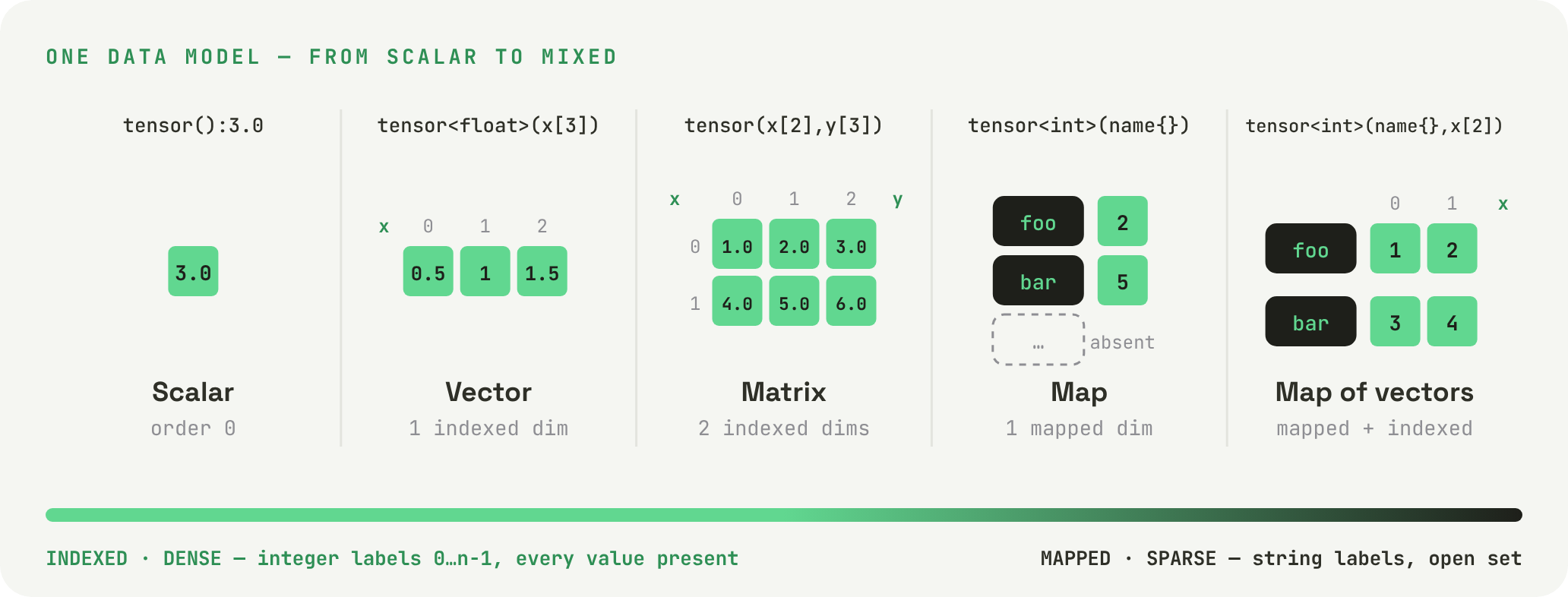
Diagram titled One data model, from scalar to mixed. Five tensors drawn as cells: a scalar 3.0 of order 0, a vector of three values on one indexed dimension x, a matrix of two rows and three columns on two indexed dimensions, a map with cells foo 2 and bar 5 and an absent cell on one mapped dimension, and a map of vectors with foo 1 2 and bar 3 4. A bar along the foot runs from indexed and dense, integer labels with every value present, to mapped and sparse, string labels in an open set. Enlarge
Figure 5. The five example tensors above, drawn. Dense and sparse dimensions share one model and can be mixed in a single tensor.
Diagram titled One data model, from scalar to mixed. Five tensors drawn as cells: a scalar 3.0 of order 0, a vector of three values on one indexed dimension x, a matrix of two rows and three columns on two indexed dimensions, a map with cells foo 2 and bar 5 and an absent cell on one mapped dimension, and a map of vectors with foo 1 2 and bar 3 4. A bar along the foot runs from indexed and dense, integer labels with every value present, to mapped and sparse, string labels in an open set.

5.3

Tensor functions


The following nine functions define the language of computation over tensors:

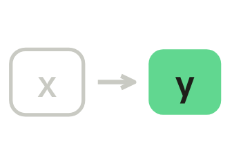
  1. 5.3.1 map Apply a lambda to every cell
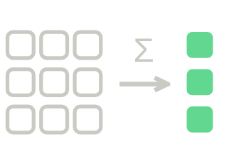
  2. 5.3.2 reduce Aggregate away dimensions
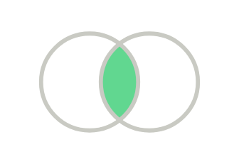
  3. 5.3.3 join Natural join on shared dimensions
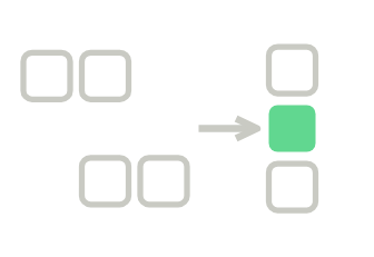
  4. 5.3.4 merge Union of cells; a lambda resolves overlaps
  5. 5.3.5 rename Change dimension names
  6. 5.3.6 concat Append along an indexed dimension
  7. 5.3.7 tensor Generate a bound tensor from a lambda
  8. 5.3.8 slice Select cells by partial address
  9. 5.3.9 tensor-literal-form Create a tensor from literal cells
Figure 6. The language of computation at a glance. Every composite function in Table 1 is built from these.

5.3.1

Function: map

map(tensor1, f(x)(expression))

A tensor with the lambda function defined by f(x)(expression) applied to each cell value of tensor1, where expression is a regular mathematical expression over scalars.

The type of this tensor is the same as tensor1.

5.3.2

Function: reduce

reduce(tensor1, aggregator, dim1, dim2, ...)

A tensor with the aggregator applied over all values of the given dimensions to produce a single value for each point of tensor1 in its remaining dimensions.

The type of this tensor is the set of dimensions in the type of tensor1 which are not in the given list of dimensions. If no dimensions are specified, this reduces over all dimensions, producing a dimensionless tensor (a scalar).

Aggregators:

  • avg: arithmetic mean
  • count: number of elements
  • prod: product of all values
  • sum: sum of all values
  • max: maximum value
  • min: minimum value

5.3.3

Function: join

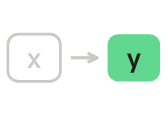
join(tensor1, tensor2, f(x,y)(expression))

A tensor constructed from the natural join between tensor1 and tensor2, with the resulting cells having the value defined by f(x,y)(expression), where x is the cell value from tensor1 and y from tensor2.

The type of this tensor has the union of dimension of tensor1 and tensor2, where the size of any bound dimension present in both is the minimum of their sizes. The cells are the set of all combinations of cells that have equal values on their common dimensions.

Whenever the lambda of join has an infix operator form in regular arithmetics, a valid short form is to denote the join with that lamda by that operator, i.e join(a, b, f(x,y)(x ∗ y)) can be written as a ∗ b.

5.3.4

Function: merge

merge(tensor1, tensor2, f(x,y)(expression))

A tensor consisting of all cells from both the arguments, where the lambda function is used to produce a single value in the cases where both arguments provide a value for a cell. The arguments must have the same types.

5.3.5

Function: rename

rename(tensor1, dimensionsToRename, newNames)

Renames one or more dimensions in the tensor. The second and third argument must have the same length and can either be a single dimension name or a list of dimension names enclosed in parenthesis. The type of the resulting tensor is the same as that of tensor1, with the names of the specified dimensions changed.

5.3.6

Function: concat

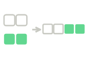
concat(tensor1, tensor2, dim)

Concatenates two tensors along the indexed dimension dim, such that any values in tensor2 have indexes in that dimension starting at the next index after the last value in that dimension in tensor1. If the dimension dim is not present in an argument tensor, all its values are taken to lie at the first index in that dimension.

The type of this tensor is the union of the types of tensor1 and tensor2, where the size of any bound dimension present in both is the max of their sizes, and where the dimension dim is added as a bound indexed dimension having the size of the sum of this dimension in tensor1 and tensor2, and the size is taken to be 1 if the dimension is missing.

This definition allows tensors of different sizes to be concatenated and when this occurs, missing values are padded with zeros.

5.3.7

Function: tensor

tensorType(expression)

Defines a new tensor according to type specification and lamba expression body expression.

The type of this tensor is the bound indexed tensor given by tensorType. expression will be evaluated for each cell implied by the type. The arguments of the expression are the names of the dimensions defined in the type spec (therefore, the lambda heading is omitted).

5.3.8

Function: slice

(tensor1){partial-address}

Slices a tensor by returning a tensor containing all the cells matching the partial address, with a type consisting of the dimensions of the argument which are not specified in the partial address. Address indexes may be supplied by a lambda function.

5.3.9

Function: tensor-literal-form

tensor-type : tensor-cells

Creates a tensor from a type and cell values given literally. Each cell value may be supplied by a lambda function.

By combining join and rename any such semantics can be achieved for any tensors.

— SECTION 6

6

Discussion


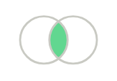
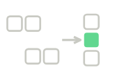
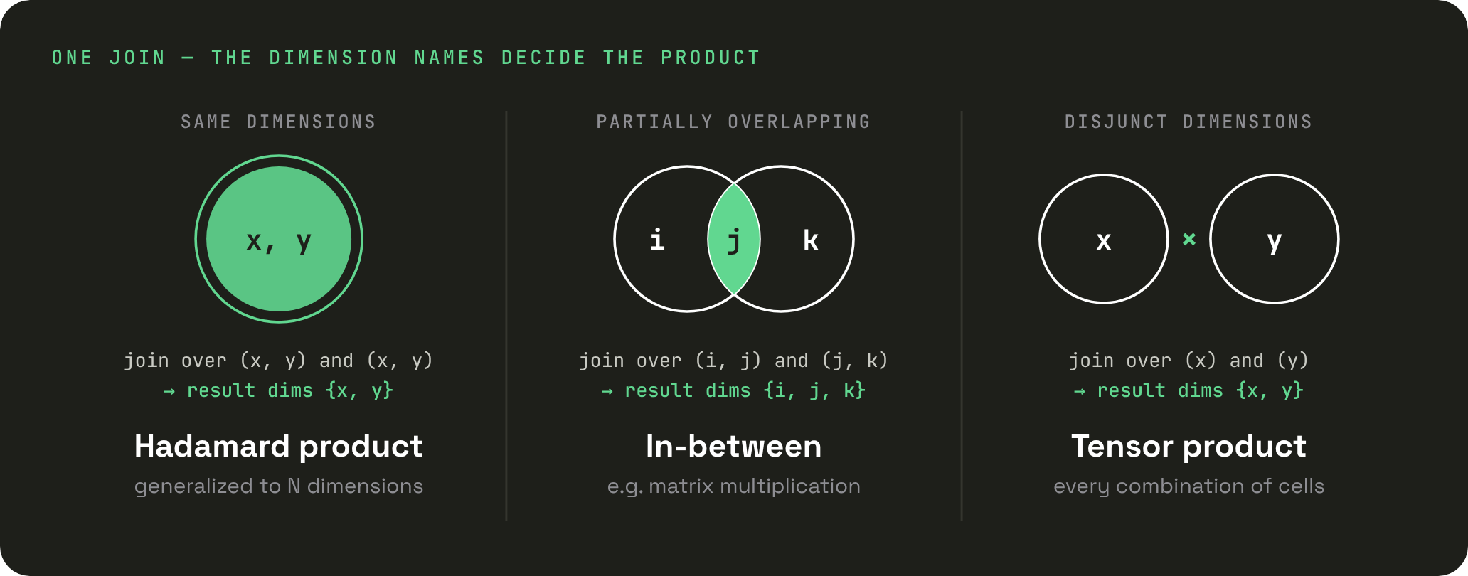
The tensor functions defined in the previous section provide a language which allows general computation to be expressed over any combination of sparse (mapped) and dense (indexed) tensor dimensions. Much of the expressible power of the model is due to using lambdas, but in addition it is also due to the generality of join resulting from the use of named dimensions: A join over tensors with the same dimensions is mathematically the matrix Hadamard product generalized to N dimensions, while a join over disjunct dimensions is the tensor product. A join over partially overlapping dimensions produces results in-between these extremes (of which matrix multiplication is a well-known example). By combining join and rename any such semantics can be achieved for any tensors.

Diagram titled One join, the dimension names decide the product. Three pairs of circles. Same dimensions: join over (x, y) and (x, y) gives result dims {x, y}, the Hadamard product generalized to N dimensions. Partially overlapping: join over (i, j) and (j, k) gives {i, j, k}, in-between, for example matrix multiplication. Disjunct dimensions: join over (x) and (y) gives {x, y}, the tensor product, every combination of cells. Enlarge
Figure 7. With named dimensions, a single join spans the Hadamard product, matrix multiplication and the tensor product.
Diagram titled One join, the dimension names decide the product. Three pairs of circles. Same dimensions: join over (x, y) and (x, y) gives result dims {x, y}, the Hadamard product generalized to N dimensions. Partially overlapping: join over (i, j) and (j, k) gives {i, j, k}, in-between, for example matrix multiplication. Disjunct dimensions: join over (x) and (y) gives {x, y}, the tensor product, every combination of cells.

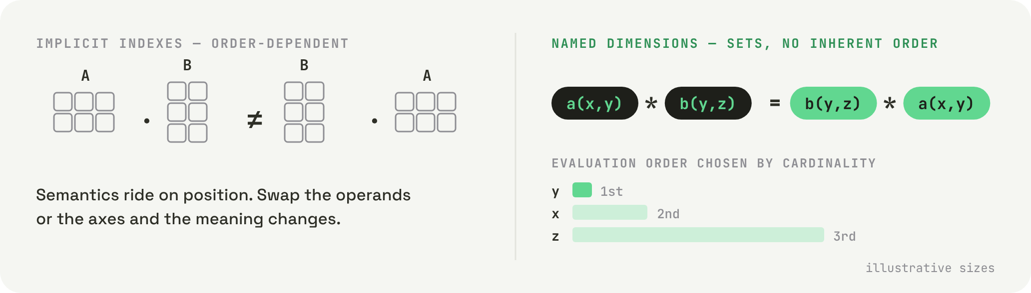
A further consequence of using named dimensions is that tensor computation becomes not only associative but also commutative. In mathematics tensor operations are not necessarily commutative since the semantics of operations are defined by the implicit indexes of the dimensions, which are order dependent. By using named dimension and defining tensors and their types in terms of sets, which are inherently unordered, commutativity is trivially achieved (the exception is concat, which has an explicitly order-dependent definition). This makes it easier to work with tensors expressions for humans but also opens up important opportunities for optimization, as it is often beneficial to perform computation in an order chosen by the cardinality of the dimensions instead of the given order.

Two panels. Left, titled Implicit indexes, order-dependent: grids A times B drawn as not equal to B times A, over the note Semantics ride on position. Swap the operands or the axes and the meaning changes. Right, titled Named dimensions, sets, no inherent order: a(x,y) * b(y,z) equals b(y,z) * a(x,y), and an evaluation order chosen by cardinality, y first, x second, z third, marked illustrative sizes. Enlarge
Figure 8. Defining types as sets of named dimensions makes computation commutative, freeing the engine to choose the evaluation order.
Two panels. Left, titled Implicit indexes, order-dependent: grids A times B drawn as not equal to B times A, over the note Semantics ride on position. Swap the operands or the axes and the meaning changes. Right, titled Named dimensions, sets, no inherent order: a(x,y) * b(y,z) equals b(y,z) * a(x,y), and an evaluation order chosen by cardinality, y first, x second, z third, marked illustrative sizes.

By allowing string labels as indexes, we can represent string based models without resorting to storing strings in place of scalar values. In this way, the universality of functions can be maintained also for models operating on string data. Since the type produced by each function is clearly defined, the type resulting from any computation is readily computed statically by composition.

6.1

Higher-order functions


Table 1 (next page) lists a set of commonly used tensor functions and their definition in terms of the language of functions listed above.

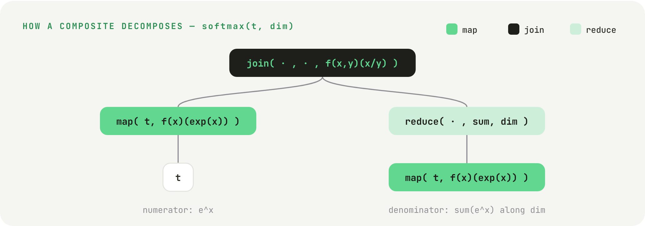
Tree diagram titled How a composite decomposes, softmax(t, dim). The root, join( · , · , f(x,y)(x/y) ), has two branches. The numerator is map( t, f(x)(exp(x)) ) over t. The denominator is reduce( · , sum, dim ) over map( t, f(x)(exp(x)) ). A legend colours map, join and reduce. Enlarge
Figure 9. softmax, as defined in Table 1, is a tree of three core functions.
Tree diagram titled How a composite decomposes, softmax(t, dim). The root, join( · , · , f(x,y)(x/y) ), has two branches. The numerator is map( t, f(x)(exp(x)) ) over t. The denominator is reduce( · , sum, dim ) over map( t, f(x)(exp(x)) ). A legend colours map, join and reduce.

Table 1. Composite functions and their formal definition


TABLE 1 ROWS USING EACH CORE FUNCTION
Figure 10. Counted from the definitions in Table 1; a row can use more than one core function.
FUNCTIONFORMAL DEFINITIONDESCRIPTIONCORE
abs(t) map(t, f(x)(abs(x))) Absolute value of all elements.
  • map
acos(t) map(t, f(x)(acos(x))) Arc cosine of all elements.
  • map
t1 + t2 join(t1, t2, f(x, y)(x + y)) Join and sum tensors t1 and t2.
  • join
argmax(t) join(t, max(t), f(x, y)(if(x == y, 1, 0))) A tensor with cell(s) of the highest value(s) in the tensor set to 1.
  • join
argmin(t) join(t, min(t), f(x, y)(if(x >= y, 0, 1))) A tensor with cell(s) of the lowest value(s) in the tensor set to 1.
  • join
asin(t) map(t, f(x)(asin(x))) Arc sine of all elements.
  • map
atan(t) map(t, f(x)(atan(x))) Arc tangent of all elements.
  • map
atan2(t1, t2) join(t1, t2, f(x, y)(atan2(x, y))) Arctangent of t1 and t2.
  • join
avg(t, dim) reduce(t, avg, dim) Reduce the tensor with the average aggregator along dimension dim.
  • reduce
ceil(t) map(t, f(x)(ceil(x))) Ceiling of all elements.
  • map
count(t, dim) reduce(t, count, dim) Reduce the tensor with the count aggregator along dimension dim.
  • reduce
cos(t) map(t, f(x)(cos(x))) Cosine of all elements.
  • map
cosh(t) map(t, f(x)(cosh(x))) Hyperbolic cosine of all elements.
  • map
diag(n1, n2) tensor(i[n1], j[n2])(if(i == j, 1.0, 0.0))) A tensor with the diagonal set to 1.0.
  • tensor
t1/t2 join(t1, t2, f(x, y)(x/y)) Join and divide tensors t1 and t2.
  • join
elu(t) map(t, f(x)(if(x < 0, exp(x) − 1, x))) Exponential linear unit.
  • map
t1 == t2 join(t1, t2, f(x, y)(x == y)) Join and determine if each element in t1 and t2 are equal.
  • join
exp(t) map(t, f(x)(exp(x))) Exponential function (ex) of each element.
  • map
floor(t) map(t, f(x)(floor(x))) Floor of each element.
  • map
t1 > t2 join(t1, t2, f(x, y)(x > y)) Join and determine if each element in t1 is greater than t2.
  • join
t1 >= t2 join(t1, t2, f(x, y)(x >= y)) Join and determine if each element in t1 is greater than or equals t2.
  • join
t1 < t2 join(t1, t2, f(x, y)(x < y)) Join and determine if each element in t1 is less than t2.
  • join
t1 <= t2 join(t1, t2, f(x, y)(x <= y)) Join and determine if each element in t1 is less than or equals t2.
  • join
l1_normalize(t, dim) join(t, reduce(t, sum, dim), f(x, y)(x/y)) L1 normalization: t/sum(t, dim).
  • join
  • reduce
l2_normalize(t, dim) join(t, map(reduce(map(t, f(x)(x ∗ x)), sum, dim), f(x)(sqrt(x))), f(x, y)(x/y)) L2 normalization: t/sqrt(sum(t2, dim).
  • map
  • join
  • reduce
log(t) map(t, f(x)(log(x))) Natural logarithm of each element.
  • map
log10(t) map(t, f(x)(log10(x))) Logarithm with base 10 of each element.
  • map
matmul(t1, t2, dim) reduce(join(t1, t2, f(x, y)(x ∗ y)), sum, dim) Matrix multiplication of two tensors. This is the product of the two tensors summed along a shared dimension.
  • join
  • reduce
max(t, dim) reduce(t, max, dim) Reduce the tensor with the max aggregator along dimension dim.
  • reduce
max(t1, t2) join(t1, t2, f(x, y)(max(x, y))) Join and return the max of t1 or t2. Arguments can be scalars.
  • join
min(t, dim) reduce(t, min, dim) Reduce the tensor with the min aggregator along dimension dim.
  • reduce
min(t1, t2) join(t1, t2, f(x, y)(min(x, y))) Join and return the minimum of t1 or t2. Arguments can be scalars.
  • join
mod(t, constant) map(t, f(x)(mod(x, constant))) Modulus of constant with each element.
  • map
t1 ∗ t2 join(t1, t2, f(x, y)(x ∗ y)) Join and multiply tensors t1 and t2.
  • join
t1 != t2 join(t1, t2, f(x, y)(x != y)) Join and determine if each element in t1 and t2 are not equal.
  • join
pow(t, constant) map(t, f(x)(pow(x, constant))) Raise each element to the power of constant.
  • map
prod(t, dim) reduce(t, prod, dim) Reduce the tensor with the product aggregator along dimension dim.
  • reduce
random(n1, n2, ...) tensor(i1[n1], i2[n2], ...)(random(1.0)) A tensor with random values between 0.0 and 1.0, uniform distribution.
  • tensor
range(n) tensor(i[n])(i) A tensor with increasing values.
  • tensor
relu(t) map(t, f(x)(max(0, x))) Rectified linear unit.
  • map
round(t) map(t, f(x)(round(x))) Round each element.
  • map
sigmoid(t) map(t, f(x)(1.0/(1.0 + exp(0.0 − x)))) The sigmoid of each element.
  • map
sin(t) map(t, f(x)(sin(x))) Sinus of each element.
  • map
sinh(t) map(t, f(x)(sinh(x))) Hyperbolic sinus of each element.
  • map
sign(t) map(t, f(x)(if(x < 0, −1.0, 1.0))) The sign of each element.
  • map
softmax(t, dim) join(map(t, f(x)(exp(x))), reduce(map(t, f(x)(exp(x))), sum, dim), f(x, y)(x/y)) The softmax of the tensor, e.g. ex/sum(ex).
  • map
  • join
  • reduce
sqrt(t) map(t, f(x)(sqrt(x))) The square root of each element.
  • map
square(t) map(t, f(x)(square(x))) The square of each element.
  • map
t1 − t2 join(t1, t2, f(x, y)(x − y)) Join and subtract tensors t1 and t2.
  • join
sum(t, dim) reduce(t, sum, dim) Reduce the tensor with the summation aggregator along dimension dim.
  • reduce
tan(t) map(t, f(x)(tan(x))) The tangent of each element.
  • map
tanh(t) map(t, f(x)(tanh(x))) The hyperbolic tangent of each element.
  • map
xw_plus_b(x, w, b, dim) join(reduce(join(x, w, f(x, y)(x ∗ y)), sum, dim), b, f(x, y)(x + y)) Matrix multiplication of x (usually a vector) and w (weights), with b added (bias).
  • join
  • reduce

6.2

Model examples


To give some flavor of how this language can be used in practice, we show two examples.

First, a neural net with one hidden layer (expressed in the composite functions listed in the table on the next page):

TENSORS:

inputTensor:        tensor(input[20])
hiddenLayerWeights: tensor(input[20],hidden[40])
hiddenLayerBias:    tensor(hidden[40])
finalLayerWeights:  tensor(hidden[40], final[1])
finalLayerBias:     tensor(final[1])

EXPRESSION:

sigmoid(sum(relu(sum(inputTensor *
                     hiddenLayerWeights, input)
             + hiddenLayerBias)
             * finalLayerWeights, hidden)
          + finalLayerBias)

EVALUATION, WITH THE TYPE OF EVERY INTERMEDIATE

type function

  1. INPUTTENSORinput[20]
  2. ∗hiddenLayerWeights
  3. TYPEinput[20],hidden[40]
  4. sumover input
  5. TYPEhidden[40]
  6. +hiddenLayerBias
  7. relu
  8. TYPEhidden[40]
  9. ∗finalLayerWeights
  10. TYPEhidden[40],final[1]
  11. sumover hidden
  12. TYPEfinal[1]
  13. +finalLayerBias
  14. sigmoid
  15. OUTPUTfinal[1]
Figure 11. The neural net expression evaluated step by step. Each intermediate type follows statically from the function that produced it.

Second, a regression model which supplies a weight for each combination of three sparse feature vectors (using the short form of join):

TENSORS:

topics:         tensor(topic{})
interests:      tensor(interest{})
locations:      tensor(location{})
learnedWeights: tensor(topic{},
                       interest{},
                       location{})

EXPRESSION:

sum(
  topics * interests * locations // Combine features
  * learnedWeights               // Apply weights
)

SUM( TOPICS * INTERESTS * LOCATIONS * LEARNEDWEIGHTS )

    1. topicstopic{}
    2. interestsinterest{}
    3. locationslocation{}
  1. ∗ ∗// Combine features
  2. TYPEtopic{},interest{},location{}
  3. ∗learnedWeights// Apply weights
  4. sum
  5. SCALARtensor()
Figure 12. The sparse regression model: join three sparse feature vectors, apply learned weights, sum to a score.

7

Current applications


This formalism is adopted for scalable inference during query evaluation in the Vespa.ai big data serving engine [4]. It is used for two purposes: As a language for practitioners to express their models, and as a common runtime inference engine both for models expressed directly in this language and models imported from TensorFlow [5] and Onnx [6] representations. This is a good indication of the generality of the formalism, and in practical terms means that Vespa developers can focus their attention on optimizing a single runtime to improve performance on models written in all these forms (as well as any combination such as writing an expression combining multiple TensorFlow models).

Such models have been running for some time in production to perform tensor based inferences at large scale in various applications, such as neural nets for user comment ranking [7], and various embedded vector similarity scoring models.

A complete standalone implementation in Java of the tensor formalism described here is also available in open source on GitHub [8].

FROM FORMALISM TO PRODUCTION

    • Tensor language

      models expressed directly in this language

    • TensorFlow [5]

      imported models

    • Onnx [6]

      imported models

  1. ONE RUNTIME

    Common runtime inference engine

    optimize a single runtime to improve performance on models written in all these forms

    • map
    • reduce
    • join
    • merge
    • rename
    • concat
    • tensor
    • slice
    • literal
  2. QUERY EVALUATION

    Vespa.ai big data serving engine [4]

    • Neural nets [7]

      for user comment ranking

    • Vector similarity

      various embedded scoring models

Scalable inference during query evaluation

Open source Java implementation on GitHub [8]

Figure 13. How the formalism runs in Vespa.ai: three ways to express a model, one runtime to optimize, in production during query evaluation.

8

Conclusion


Basing numerical computation on tensors promises interoperability, ease of abstraction, and meta-reasoning over computation. However, to deliver on this promise rather than becoming just an inconvenient data structure for communication between arbitrary pieces of code, a strong foundation for tensors and their computation is needed.

This paper has presented a formalism which provides generic computation over both dense and sparse tensors, with with full static type inference, using just six foundational tensor functions. Named dimensions are used to add semantic information and achieve generality, and index labels provide support for models working with strings. This formalism is validated in a wide range of production use cases by its adoption. By adopting this formalism, tensor frameworks and tools can deliver on the promise of tensors to make numerical computation easier to express, understand, optimize and interchange.

  • 1 model

    generic computation over both dense and sparse tensors

  • 6

    foundational tensor functions

  • Full

    static type inference